Model Training Panel
The Model Training panel contains on Inputs tab — on which you can add the required training data and select a mask, as well as set the data augmentation and validation settings — and a Training Parameters tab — on which you can define the training parameters.
Click the Go to Training button on the Deep Learning Tool dialog to open the Model Training panel, shown below. You should note that the selected model must be loaded to enable the 'Go to Training' button.
Model Training panel

The information presented on the Model Training panel, and all other panels, is associated with the currently selected deep learning model (see Model Overview Panel).
|
|
Description |
|---|---|
|
Model |
Indicates the currently selected model. |
|
Inputs |
Lets you choose a training set(s), as well as set the data augmentation and validation settings (see Inputs). |
|
Training Parameters |
Includes a set of basic settings for training a deep model, as well as advanced settings related to the selected optimization algorithm and metric and callback functions (see Training Parameters). |
|
Train |
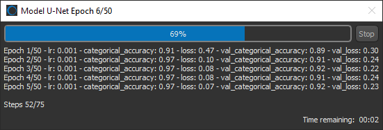
Starts the training process. Available only after the required inputs and outputs have been added in the Training Data box (see Training Data). As shown below, you can view and evaluate the training results after each epoch is completed.
You should note that training can range from a few minutes for a small network with a limited number of epochs and a small dataset to a few hours or even days for a deeper network with many epochs and a large dataset. Note After a model is successfully trained, you can process the original dataset or other similar datasets in the Image Processing Toolbox (see Comprehensive Filters), as well as in the Segment with Classifier panel (see Segment with AI). |
|
Preview |
Once training is partially or fully complete, you can preview the result of applying the model to a selected dataset (see Previewing Training Results). Note If the results are unsatisfactory, you can continue training with new inputs and/or parameters and concentrate on problematic areas. Once you are satisfied with the results, you can save the model and close the Deep Learning Tool. |
You can choose the inputs for training — the training input(s), output(s), and masks — as well as select the data augmentation and validation settings on the Inputs tab. Click the Inputs tab on the Model Training panel to go to the Inputs tab, shown below.
Inputs tab

A. Training Data B. Data Augmentation settings C. Validation settings
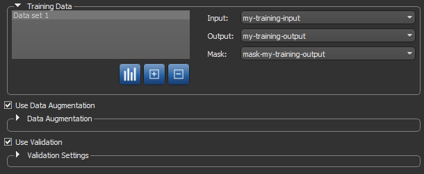
You can choose the training input(s), an output, and a mask for defining the model working space in the Training Data box, shown below.
Training Data
|
|
Description |
|---|---|
|
Training Data list |
Lists all of the selected training sets, which include inputs, outputs, and masks. Options in the Training Data list include the following: Show Training Data Statistics… Click the Show Statistics
Note This option is NOT available for regression models. Add New Training Dataset… Click the Add New
Remove New Training Dataset… Click the Remove |
|
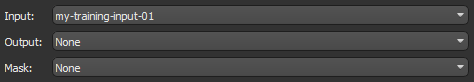
Input |
Lets you select the training input(s). In simple cases, you will only have to choose a single input, as shown below. In other cases, such as when you work with multi-slice inputs or multiple inputs, selecting additional settings is required.
Note If you selected '3D' as the input dimension in the Model Generator dialog, then additional options will be available for the training input (see Configuring Multi-Slice Inputs). Note You can also choose to multiple inputs for the training input. For example, when you are working with data from simultaneous image acquisition systems (see Model Training Panel). |
|
Output |
Lets you select a target output for training. You should note that outputs are dependent on the type of model that will be trained and must be same size and shape as the input data for training semantic segmentation and denoising models. Outputs for super-resolution can be a factor — 2, 4, or 8 times — of the input X-Y dimension. If you are training a model for continuous output, for example with an autoencoder for denoising or super-resolution, you have to select an image channel as the output. If you are training a model for semantic segmentation, you will need to select a multi-ROI with the same number of classes as the model's 'class count' (see Model Generator). |
|
Lets you select a mask to define the working space for the model, which can help reduce training times and increase training accuracy. You should note that masks should be large enough to enclose the input (patch) size and that rectangular shapes are often best. See Applying Masks for additional information about mask requirements. |
|
|
Use Data Augmentation |
If selected, data augmentation will be applied during training (see Data Augmentation Settings). Data augmentation is a technique that can be used to artificially expand the size of a training dataset by creating modified versions of the images in the dataset Note The current data augmentation settings are applied to all new models by default. |
|
Use Validation |
If selected, validation will be applied during training (see Validation Settings). Note The current validation settings are applied to all new models by default, except those related to designated data. |
 button to open the Training Data Statistics dialog, shown below. The dialog, which is available for segmentation models only, lists the total number of voxels in the training set(s) added to the model, the percentage of labeled training voxels, and the percentage of labeled voxels associated with each class. Cumulative statistics for all training data is also presented. You should note that 'Class 1' is always associated with the background, and that all statistics are computed within selected masks.
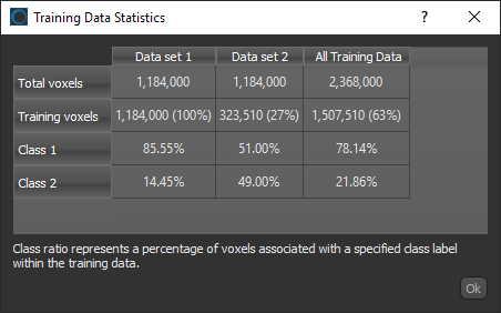
If you selected '3D' as the input dimension in the Model Generator dialog, then additional options will be available for the input dataset, as shown below.
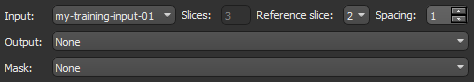
Slices… Indicates the number of slices that was entered in the Model Generator dialog for the 3D input dimension (see Model Generator).
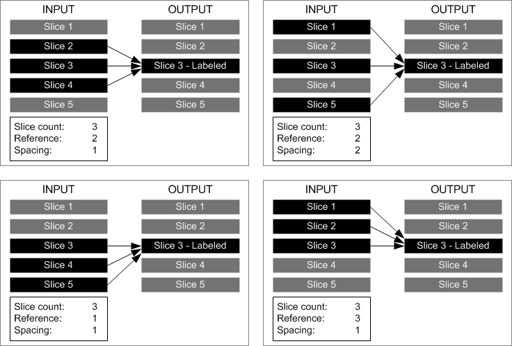
Reference slice… Lets you choose the index of the input slice that corresponds to the target output slice. For example, if the slice count is '3', the reference slice is '2', and spacing is '1', then the reference slice and the slices directly below and above the reference will be looked at when the model is trained. If the reference is changed to '1' for the same case, then the reference slice and the two slices directly below the reference will be looked at.
Spacing… Lets you choose the distance, or offset, between slices. Choosing '1' means that slices are taken sequentially, '2' means every other slice is taken, and so on. You should note that if sequential slices are very similar, then you should increase spacing. You should also note that the spacing options are limited by the size of the input dataset. For example, if the input dataset has 20 slices and the number of slices is 3, then the maximum spacing possible will be 9.
The following examples illustrate the effect of selecting different input settings.
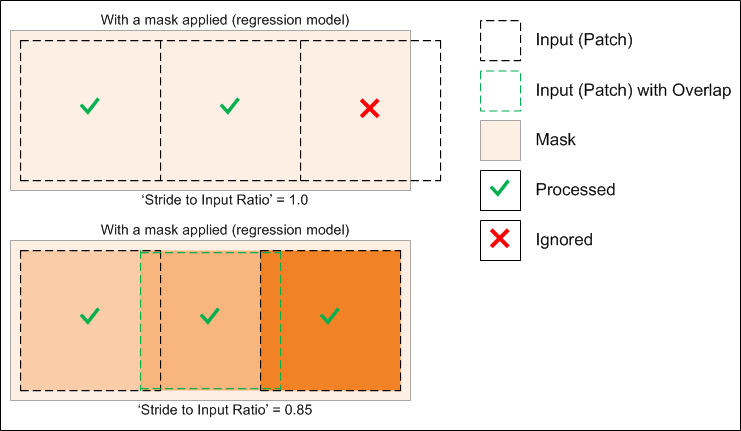
Masks let you define the working space for the model, which can help reduce training times and increase training accuracy. You should note that masks should be large enough to enclose the input (patch) size and that rectangular shapes are often best.
The starting point of the input (patch) grid is calculated from the minimum (0,0) of each connected component in the mask. You should note that for both segmentation and regression models, input (patches) that do not correspond 100% with the applied mask will be ignored during training, as shown below. You should also note that in segmentation cases, patches that correspond to the applied mask, but that are not fully segmented, will be ignored during training. For example, in cases in which the background (class 1) is not labeled.
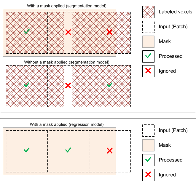
Note The selected 'Stride to Input Ratio' may affect which patches are processed. At a setting of '1.0', patches will be extracted sequentially one after another without any overlap, while at a setting less than '1.0', overlaps will be created between data patches (see Basic Settings for more information about this training parameter).
The performance of deep learning neural networks often improves with the amount of data available, particularly the ability of the fit models to generalize what they have learned to new images.
A common way to compensate small training sets is to use data augmentation. If selected, different transformations will be applied to simulate more data than is actually available. Images may be flipped vertically or horizontally, rotated, sheared, or scaled. As such, specific data augmentation options should be chosen within the context of the training dataset and knowledge of the problem domain. In addition, you should consider experimenting with the different data augmentation methods to see which ones result in a measurable improvement to model performance, perhaps with a small dataset, model, and training run.
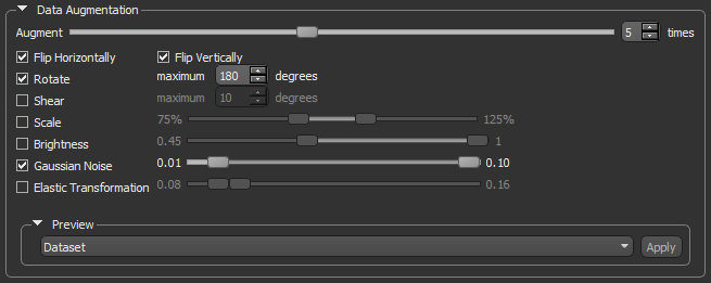
Check the Use Data Augmentation option to activate the Data Augmentation settings, shown below.
Data Augmentation settings
|
|
Description |
|---|---|
|
Augment |
Lets you choose how many times each data patch is augmented during a single training epoch. You should note that at a setting of '1', the amount of training data will be doubled, at a setting of '2', the training data will be tripled, and so on. |
|
Flip Horizontally |
Flips data patches horizontally by reversing the columns of pixels. |
|
Flip Vertically |
Flips data patches vertically by reversing the rows of pixels. |
|
Rotate |
Randomly rotates data patches clockwise by a given number of degrees from 0 to the set maximum. Maximum degrees… Lets you set the maximum number of degrees in the rotation. The maximum number of degrees that the data can be rotated is 180. |
|
Shear |
Randomly shears data patches clockwise by a given number of degrees from 0 to the set maximum. Maximum degrees… Lets you set the maximum number of degrees to shear images. The maximum number of degrees that the data can be sheared is 45. |
|
Scale |
Randomly scales the image within a specified range. For example, between 70% (zoom in) and 130% (zoom out). Note Values less than 100% will scale the image in. For example, a setting of 50% will make the objects in the image 50% larger. Values larger than 100% will zoom the image out, making objects smaller. Scaling at 100% will have no effect. |
|
Brightness |
Randomly darkens images within a specified range, for example between 0.2 or 20% and 1.0 (no change). In this case, the intent is to allow a model to generalize across images trained on different illumination levels. |
|
Gaussian Noise |
Randomly adds Gaussian noise, within a specified range, to the image. |
|
Elastic Transformation |
Randomly adds an elastic transformation, within a specified range, to the image. Note Computing elastic transformations is computationally expensive and selecting this option will likely increase training times significantly. |
|
Preview |
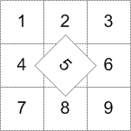
Lets you preview the effect of data augmentation on a selected training data input. Click the Apply button to preview data augmentation in the current scene. Note The original patch size is always maintained when transformations are applied, as shown in the example below for the rotation of patch 5. In this case, some data from patches 2, 4, 6, and 8 will be added to patch 5.
For border patches, the original image will be padded with extra rows and columns, as required. For example, column[-1] = column [1], column [-2] = column [2], and so on. |
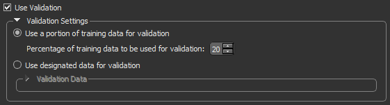
Machine learning algorithms, whether deep or not, are often prone to overfitting. Overfitting is a situation in which an algorithm just memorizes the data from training and fails to provide good results on new, previously unseen data. In order to avoid this situation, separate data can be used for algorithm validation.
In Dragonfly, you can either randomly split the available data into training and validation sets by specifying a percentage of the data to be preserved for validation, or you can provide separate validation data, which will be used only for accuracy evaluation and not for training. If you have only one dataset, you can reuse it for both training and validation by defining non-intersecting masks.
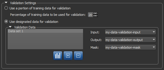
Validation settings
|
|
Description |
|---|---|
|
Use a portion of training data for validation |
Lets you automatically split the model inputs into training and validation sets. Percentage of training data to be used for validation… Lets you choose the percentage of the training data that will be used for validation. In this case, the training set will be used for neural network training and the validation set will be used only for accuracy evaluation, but not for training. |
|
Use designated data for validation |
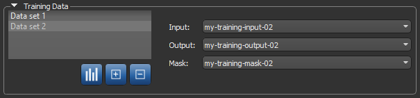
Lets you choose separate data for algorithm validation, as shown below.
Note You can use the same data for both training and validation provided that you apply non-intersecting masks. |
The Training Parameters tab, shown below, includes a set of basic settings for training a deep learning model, as well advanced settings that let you modify the default settings of the selected optimization algorithm and to add metric and callback functions.
Training Parameters tab

A. Basic settings B. Advanced settings
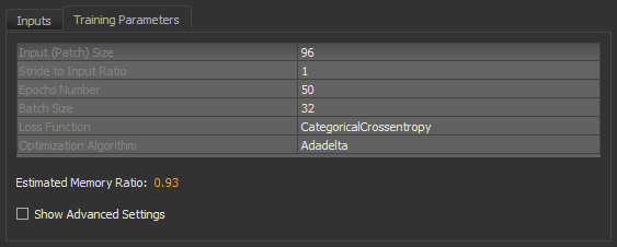
The basic settings that you need to set to train a deep learning model are available in the top section of the Training Parameters tab, as shown below.
Basic settings
|
|
Description |
|---|---|
|
Input (Patch) Size |
During training, training data is split into smaller 2D data patches, which is defined by the 'Input (Patch) Size' parameter. For example, if you choose an Input (Patch) Size of 64, the Deep Learning Tool will cut the dataset into sub-sections of 64´64 pixels. These subsections will then be used as the training dataset. By subdividing images, each pass or 'epoch' should be faster and use less memory. |
|
Stride to Input Ratio |
The 'Stride to Input Ratio' specifies the overlap between adjacent patches. At a value of '1.0', there will be no overlap between patches and they will be extracted sequentially one after another. At a value of '0.5', there will be a 50% overlap. You should note that any value greater than '1.0' will result in gaps between data patches. |
|
Epochs Number |
A single pass over all the data patches is called epoch, and the number of epochs is controlled by the 'Epochs Number' parameter. |
|
Batch Size |
Patches are randomly processed in batches and the 'Batch Size' parameter determines the number of patches in a batch. |
|
Loss Function |
Loss functions, which are selectable in the drop-down menu, measure the error between the neural network's prediction and reality. The error is then used to update the model parameters (go to www.tensorflow.org/api_docs/python/tf/keras/losses for additional information about the loss functions available in Dragonfly's Deep Learning Tool). You should note that not all the loss functions will work well with all models and the available selections are automatically filtered according to the model type — Regression (for super-resolution and denoising) and Semantic Segmentation (for binary and multi-class segmentations). Regressive loss functions… Are used in cases of regressive problems, that is when the target variable is continuous. One of the most widely used regressive loss functions is Mean Squared Error. Other loss functions you might consider are Cosine Similarity, Huber, Mean Absolute Error, Poisson, and others listed in the drop-down menu (see Loss Functions for Regression Models). Semantic segmentation loss functions… Are used in cases of segmentation problems, that is when the target output is a multi-ROI. When training a multi-class segmentation model, 'CategoricalCrossentropy' is generally a good choice as a classification for each pixel must be made. See Loss Functions for Semantic Segmentation Models for additional information about the available loss functions. |
|
Optimization Algorithm |
Optimization algorithms are used to update the parameters of the model so that prediction errors are minimized. Optimization is a procedure in which the gradient — the partial derivative of the loss function with respect to the network's parameters — is first computed and then the model weights are modified by a given step size in the direction opposite of the gradient until a local minimum is achieved. Dragonfly's Deep Learning Tool provides several optimization algorithms — Adagrad, Adam, RMSProp, SDG (Stochastic Gradient Descent), and many others — which work well on different kinds of problems. In many cases, Adam is generally a good starting point. The default settings can be modified in the Advanced Settings (see Optimization Algorithm Parameters). Note You can find more information about optimization algorithms at www.tensorflow.org/api_docs/python/tf/keras/optimizers. You can also refer to the publication Demystifying Optimizations for Machine Learning (towardsdatascience.com/demystifying-optimizations-for-machine-learning-c6c6405d3eea). |
|
Displays the estimated memory ratio, which is calculated as the ratio of your system's capability and the estimated memory needed to train the model at the current settings. You should note that the total memory requirements to train a model depends on the implementation and selected optimizer. In some cases, the size of the network may be bound by your system's available memory. Green … The estimated memory requirements are within your system's capabilities. Yellow … The estimated memory requirements are approaching your system's capabilities. Red … The estimated memory requirements exceed your system's capabilities. You should consider adjusting the model training parameters or selecting a shallower model. Note Memory is one of the biggest challenges in training deep neural networks. Memory is required to store input data, weight parameters and activations as an input propagates through the network. In training, activations from a forward pass must be retained until they can be used to calculate the error gradients in the backwards pass. As an example, the 50-layer ResNet network has about 26 million weight parameters and computes close to 16 million activations in the forward pass. If you use a 32-bit floating-point value to store each weight and activation this would give a total storage requirement of 168 MB. By using a lower precision value to store these weights and activations you could halve or even quarter this storage requirement. Note Refer to imatge-upc.github.io/telecombcn-2016-dlcv/slides/D2L1-memory.pdf for information about calculating memory requirements. |
|
|
Show Advanced Settings |
If selected, lets you access the Advanced Settings panel (see Advanced Settings). |
The following loss functions are available for regression models.
|
|
Description |
|---|---|
|
CosineSimilarity |
Computes the cosine similarity between Reference: https://www.tensorflow.org/api_docs/python/tf/keras/losses/CosineSimilarity |
|
Huber |
Computes the Huber loss between Reference: www.tensorflow.org/api_docs/python/tf/keras/losses/Huber |
|
LogCosh |
Computes the logarithm of the hyperbolic cosine of the prediction error. Reference: www.tensorflow.org/api_docs/python/tf/keras/losses/LogCosh |
|
MeanAbsoluteError |
Computes the mean absolute difference between the labels and predictions. Reference: www.tensorflow.org/api_docs/python/tf/keras/losses/MeanAbsoluteError |
|
MeanAbsolutePercentageError |
Computes the mean absolute percentage error between Reference: www.tensorflow.org/api_docs/python/tf/keras/losses/MeanAbsolutePercentageError |
|
MeanSquaredError |
Computes the mean of squares of error between labels and predictions. Reference: www.tensorflow.org/api_docs/python/tf/keras/losses/MeanSquaredError |
|
MeanSquaredLogarithmicError |
Computes the mean squared logarithmic error between Reference: www.tensorflow.org/api_docs/python/tf/keras/losses/MeanSquaredLogarithmicError |
|
Poission |
Computes the Poisson loss between Reference: www.tensorflow.org/api_docs/python/tf/keras/losses/Poisson |
The following loss functions are available for semantic segmentation models.
|
|
Description |
|---|---|
|
CategoricalCrossentropy |
Computes the crossentropy loss between labels and predictions. Reference: www.tensorflow.org/api_docs/python/tf/keras/losses/CategoricalCrossentropy |
|
CategoricalHinge |
Computes the categorical hinge loss between Reference: www.tensorflow.org/api_docs/python/tf/keras/losses/CategoricalHinge |
|
CosineSimilarity |
Computes the cosine similarity between the Reference: www.tensorflow.org/api_docs/python/tf/keras/losses/CosineSimilarity |
|
KLDivergence |
Computes a Kullback-Leibler divergence loss between Reference: www.tensorflow.org/api_docs/python/tf/keras/losses/KLDivergence |
|
OrsDiceLoss* |
Computes the similarity of two samples. |
|
OrsJaccardDistance* |
Computes the similarity and diversity of sample sets. Reference: en.wikipedia.org/wiki/Jaccard_index |
* The 'OrsDiceLoss' and 'OrsJaccardDistance' loss functions are often used when segmentation classes are unbalanced as they give all classes equal weight. However, you may note that training with these loss functions might be more unstable than with others. Refer to Salehi et al. Tversky loss function for image segmentation using 3D fully convolutional deep networks, Cornell University, 2017-06-17 (arxiv.org/pdf/1706.05721.pdf) for information about the implementation of these loss functions.
The following optimization algorithms are available for deep models. You should note that you can fine-tune the hyperparameters of the selected optimization algorithm to further enhance model accuracy (see Optimization Algorithm Parameters).
|
|
Description |
|---|---|
|
Adadelta |
Optimizer that implements the Adadelta algorithm. Adadelta optimization is a stochastic gradient descent method that is based on adaptive learning rate per dimension to address two drawbacks — the continual decay of learning rates throughout training, and the need for a manually selected global learning rate. Reference: www.tensorflow.org/api_docs/python/tf/keras/optimizers/Adadelta |
|
Adagrad |
Optimizer that implements the Adagrad algorithm. Adagrad is an optimizer with parameter-specific learning rates, which are adapted relative to how frequently a parameter gets updated during training. The more updates a parameter receives, the smaller the updates. Reference: www.tensorflow.org/api_docs/python/tf/keras/optimizers/Adagrad |
|
Adam |
Optimizer that implements the Adam algorithm. In many cases, Adam is generally a good starting point. Reference: www.tensorflow.org/api_docs/python/tf/keras/optimizers/Adam |
|
Adamax |
Optimizer that implements the Adamax algorithm, which is a variant of Adam based on the infinity norm. Adamax is sometimes superior to Adam, specially in models with embeddings. Reference: www.tensorflow.org/api_docs/python/tf/keras/optimizers/Adamax |
|
Nadam |
Optimizer that implements the Nadam algorithm, which is Adam with Nesterov momentum. Reference: www.tensorflow.org/api_docs/python/tf/keras/optimizers/Nadam |
|
RMSprop |
Optimizer that implements the RMSprop algorithm. Reference: www.tensorflow.org/api_docs/python/tf/keras/optimizers/RMSprop |
|
SGD |
Stochastic gradient descent and momentum optimizer. Reference: www.tensorflow.org/api_docs/python/tf/keras/optimizers/SGD |
The advanced settings let you modify the default settings of the selected optimization algorithm and to add metric and callback functions.
If required, your can fine-tune the hyperparameters of the selected optimization algorithm further enhance model accuracy. A hyperparameter is a parameter whose value is used to control the learning process. By contrast, the values of other parameters, typically node weights, are learned.
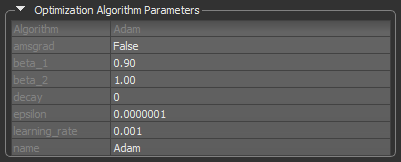
Options to set the hyperparameters of the selected optimization algorithm are available in the Optimization Algorithm Parameters box, as shown below.
Default settings for the Adam optimization algorithm
|
|
Description |
|---|---|
|
Algorithm |
Indicates the optimization algorithm selected for model training. |
|
Parameters |
The parameters of the selected optimization algorithm appear here. You can find a description of each argument for the available algorithms as follows: Adadelta… https://www.tensorflow.org/api_docs/python/tf/keras/optimizers/Adadelta#args. Adagrad… https://www.tensorflow.org/api_docs/python/tf/keras/optimizers/Adagrad#args. Adam… https://www.tensorflow.org/api_docs/python/tf/keras/optimizers/Adam#args. Adamax… https://www.tensorflow.org/api_docs/python/tf/keras/optimizers/Adamax#args. Nadam… https://www.tensorflow.org/api_docs/python/tf/keras/optimizers/Nadam#args. RMSprop… https://www.tensorflow.org/api_docs/python/tf/keras/optimizers/RMSprop#args. SGD… https://www.tensorflow.org/api_docs/python/tf/keras/optimizers/SGD#args. |
|
Name |
Optional name prefix for the operations created when applying gradients. Defaults to the name of the selected optimization algorithm, for example, Note This parameter is not available for the Adadelta and SGD optimization algorithms. |
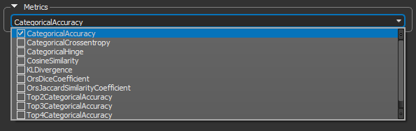
Metrics are functions that can be used to judge the performance of your model and are to be supplied when a model is compiled or evaluated. The available metrics for estimating a model's performance are available in the Metrics drop-down menu, as shown below.
Metrics
The following options are available for judging the performance of regression models.
|
|
Description |
|---|---|
|
CosineSimilarity |
Computes the cosine similarity between the labels and predictions. Reference: www.tensorflow.org/api_docs/python/tf/keras/metrics/CosineSimilarity. |
|
LogCoshError |
Computes the logarithm of the hyperbolic cosine of the prediction error. Reference: www.tensorflow.org/api_docs/python/tf/keras/metrics/LogCoshError. |
|
MeanAbsoluteError |
Computes the mean absolute error between the labels and predictions. Reference: www.tensorflow.org/api_docs/python/tf/keras/metrics/MeanAbsoluteError. |
|
MeanAbsolutePercentageError |
Computes the mean absolute percentage error between Reference: www.tensorflow.org/api_docs/python/tf/keras/metrics/MeanAbsolutePercentageError. |
|
MeanRelativeError |
Computes the mean relative error by normalizing with the given values. Reference: www.tensorflow.org/api_docs/python/tf/keras/metrics/MeanRelativeError. |
|
MeanSquaredError |
Computes the mean squared error between Reference: www.tensorflow.org/api_docs/python/tf/keras/metrics/MeanSquaredError. |
|
MeanSquaredLogarithmicError |
Computes the mean squared logarithmic error between Reference: www.tensorflow.org/api_docs/python/tf/keras/metrics/MeanSquaredLogarithmicError. |
|
Poission |
Computes the Poisson metric between Reference: www.tensorflow.org/api_docs/python/tf/keras/metrics/Poisson. |
|
RootMeanSquaredError |
Computes root mean squared error metric between Reference: www.tensorflow.org/api_docs/python/tf/keras/metrics/RootMeanSquaredError |
The following options are available for judging the performance of semantic segmentation models.
|
|
Description |
|---|---|
|
CategoricalAccuracy |
Calculates how often predictions match labels. Reference: www.tensorflow.org/api_docs/python/tf/keras/metrics/CategoricalAccuracy. |
|
CategoricalCrossentropy |
Computes the crossentropy metric between labels and predictions. Reference: www.tensorflow.org/api_docs/python/tf/keras/metrics/CategoricalCrossentropy. |
|
CategoricalHinge |
Computes the categorical hinge metric between Reference: www.tensorflow.org/api_docs/python/tf/keras/metrics/CategoricalHinge. |
|
CosineSimilarity |
Computes the cosine similarity between the labels and predictions. Reference: www.tensorflow.org/api_docs/python/tf/keras/metrics/CosineSimilarity. |
|
KLDivergence |
Computes a Kullback-Leibler divergence metric between Reference: www.tensorflow.org/api_docs/python/tf/keras/metrics/KLDivergence. |
|
OrsDiceCoefficient |
Computes a similarity metric between labels and predictions. Reference: en.wikipedia.org/wiki/Sørensen–Dice_coefficient. |
|
OrsJaccardSimilarityCoefficient |
Computes a similarity and diversity metric between labels and predictions. Reference: en.wikipedia.org/wiki/Jaccard_index. |
|
TopKCategoricalAccuracy |
Computes how often targets are in the top K (two, three, or four) predictions. Reference: www.tensorflow.org/api_docs/python/tf/keras/metrics/TopKCategoricalAccuracy. |
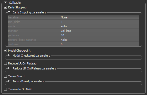
Callbacks are functions called at particular time points during the training process, usually at the end of a training epoch or at the end of batch processing. In the current version of the Deep Learning Tool, five callbacks are supported to help the training process. These are available in the Callbacks box, as shown below.
Callbacks
|
|
Description |
|---|---|
|
Early Stopping |
Stops training upon a particular condition, for example if |
|
Model Checkpoint |
Saves the model during the training (see Model Checkpoint). |
|
Reduce LR on Plateau |
Reduces the learning rate (lr) when a selected metric has stopped improving (see Reduce LR on Plateau). |
|
Terminate on NaN |
Terminates training when a NaN loss (Not a Number) is encountered. It is usually useful to select this callback, in order to stop training when a problem is encountered. Note Refer to www.tensorflow.org/api_docs/python/tf/keras/callbacks/TerminateOnNaN for more information about this callback. |
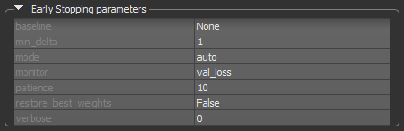
The Early Stopping callback can be set to stop training when a monitored quantity has stopped improving. This can help prevent overfitting. A good idea when using early stopping is to choose a patience level that is coherent with the selected number of epochs.
Early Stopping callback
|
|
Description |
|---|---|
|
baseline |
Is the baseline value for the monitored quantity to reach. Training will stop if the model doesn't show improvement over the baseline. |
|
min_delta |
Is the minimum change in the monitored quantity to qualify as an improvement. An absolute change of less than |
|
mode |
Determines when training will stop — Min… Training will stop when the quantity monitored has stopped decreasing. For example, when Max… Training will stop when the quantity monitored has stopped increasing. For example, when Auto… The mode — |
|
monitor |
Lets you choose the quantity to be monitored, for example, For semantic segmentation models, the quantities that can be monitored include For regression models, the quantities that can be monitored include Note Statistics related to the monitored quantities appear on the progress bar during training and in the Training Results dialog. |
|
patience |
The number of epochs with no improvement after which training will be stopped. |
|
restore_best_weights |
If |
|
verbose |
Lets you choose an option — |
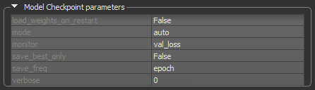
This callback can be configured to monitor a certain quantity during training and to save only the best model.
Model Checkpoint callback
|
|
Description |
|---|---|
|
load_weights_on_restart |
If |
|
mode |
Determines if the current save file should be overwritten, based on either the minimization or maximization of the monitored quantity, and |
|
monitor |
Lets you choose the quantity to be monitored, for example, For semantic segmentation models, the quantities that can be monitored include For regression models, the quantities that can be monitored include Note Statistics related to the monitored quantities appear on the progress bar during training and in the Training Results dialog. |
|
save_best_only |
If |
|
save_freq |
Determines the frequency — epoch… The callback saves the model after each epoch. Integer… The callback saves the model at end of a batch at which this many samples have been seen since last saving. Note that if the saving isn't aligned to epochs, the monitored metric may potentially be less reliable as it could reflect as little as 1 batch, since the metrics get reset every epoch. |
|
verbose |
Lets you choose an option — |
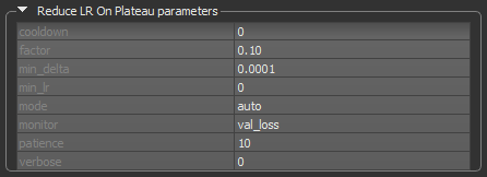
This callback can automatically reduce the learning rate of the selected optimization algorithm by a specified factor when the monitored quantity stops improving. This can be especially useful when the selected optimizer does not automatically adapt its learning rate. For example, SDG (Stochastic Gradient Descent) does not adapt automatically, but Adam does.
Reduce LR on Plateau callback
|
|
Description |
|---|---|
|
cooldown |
The number of epochs to wait before resuming normal operation after the learning rate has been reduced. |
|
factor |
The factor by which the learning rate will be reduced. Calculated as: new_lr = lr * factor. |
|
min_delta |
The threshold for measuring the new optimum, to only focus on significant changes. |
|
min_lr |
The lower bound on the learning rate. |
|
monitor |
Lets you choose the quantity to be monitored, for example, For semantic segmentation models, the quantities that can be monitored include For regression models, the quantities that can be monitored include |
|
patience |
The number of epochs with no improvement, after which learning rate will be reduced. |
|
verbose |
Lets you choose an option — |